


It is also important to remember that there are specific measures you must take when submitting/proposing a mathematical model project, such as one related to the field of biomathematics.
These steps include, but are not limited to: defining the issue, selecting a model approach (two models will be discussed in this article), formulating equations, parameter estimation—often based on historical data, implementing numerical simulations by resolving differential equations analytically or using computational tools like Python and MATLAB, validations and sensitivity analysis, scenario testing, result interpretation, and so on.
As I said earlier, this only highlights a specific step in the mathematical modeling process and employing Python for illustrative purposes.
Content Overview
- Introduction
- The Purpose of Simulation
- The SIR Model
- What It Does / SIR Python Code Simulation Example
- What You Can Learn
- Understand Disease Spread
- Explore Parameter Sensitivity
- Evaluate Interventions
- The SEIR Model
- What It Does / SEIR Python Code Simulation Example
- What You Can Learn
- Model Latent Periods
- Evaluate Early Interventions
- Study Complex Outbreaks
- Conclusion
1. Introduction
Understanding how infectious diseases spread is essential for maintaining the public’s health because they have existed throughout human history for centuries. A potent tool for simulating and understanding the dynamics of disease spread is mathematical models. The SIR (Susceptible-Infectious-Recovered) and SEIR (Susceptible-Exposed-Infectious-Recovered) models will be discussed in this article, along with how to simulate them using Python.
What Simulations Are For
For public health professionals and epidemiologists, simulation is like a crystal ball. It enables us to foresee the potential spread of diseases under various circumstances and treatment options. These models aid in decision-making, effective resource allocation, and comprehension of the potential effects of various techniques. Let’s examine two basic models namely; SIR Model, and SEIR Model.
2. The SIR Model
What It Does / SIR Python Code Simulation Example
The Susceptible, Infectious, and Recovered (SIR) model separates a population into these three categories. Based on variables like transmission rate (?) and recovery rate (?), it simulates how these compartments alter with time.
Before we exemplify a simulation using Python, it’s necessary to make “model assumptions” when working on mathematical models.
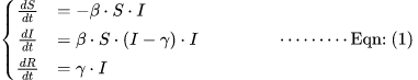
In our assumption we’ll create model using LaTeX formular or code:
\begin{align*}
\frac{dS}{dt} &= -\beta \cdot S \cdot I \\
\frac{dI}{dt} &= \beta \cdot S \cdot I - \gamma \cdot I \\
\frac{dR}{dt} &= \gamma \cdot I
\end{align*}
Note: You can latexify this formular using Python. An example can be found on https://github.com/google/latexify_py/blob/main/examples/examples.ipynb.
This article will not bother to write that Python code to convert LaTeX to a proper mathematical notation/equation, but I have used online editor such as https://latexeditor.lagrida.com/ so that you see the formula/equation assumptions glaringly below:
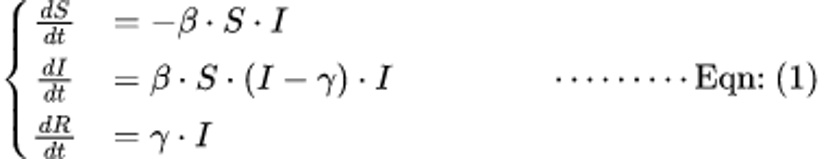
Fig 1: Model Equation
where:
- S represents susceptible individuals,
- I represents infected individuals,
- R represents recovered individuals.
The parameters ? and ? govern the rates of transmission and recovery, respectively. The negative sign (i.e ??) indicates that the number of susceptible individuals (S) decreases over time. The dot notation indicates “multiplication.”
In summary, these equations describe the dynamics of the SIR model, where the number of susceptible people decreases as they contract the disease (i.e. dS/dt), the number of infectious people rises as a result of new infections and falls as they recover (i.e. dI/dt), and the number of recovered people rises as the disease is treated (i.e. dR/dt). Because the change in each compartment depends on the multiplication of pertinent components, dots (.) is used to denote multiplication.
Since all assumptions are set, we can then run a simulation using Python for SIR Model and then visualize the dynamics:
import numpy as np
from scipy.integrate import odeint
import matplotlib.pyplot as plt

# SIR model equations
def SIR_model(y, t, beta, gamma):
    S, I, R = y
    dSdt = -beta * S * I
    dIdt = beta * S * I - gamma * I
    dRdt = gamma * I
    return [dSdt, dIdt, dRdt]


"""
Initial conditions (such as S0, I0, and R0) are not to be random but I hardcoded them with specific values. These choices are typically made based on the characteristics of the disease being modeled and the context of the simulation. Initial condition are set such that S0 = 99%, which indicates the proportion of susceptible individuals when the simulation starts. I0 is set to 1%, which indicates proportion of infected individuals to be 1% when the simulation starts. R0 is set to 0% which is expected that there are are no recovered individuals when the simulations start.
"""
S0 = 0.99
I0 = 0.01
R0 = 0.00
y0 = [S0, I0, R0]

# Parameters
# ? (beta) is transmission rate and I chose 30%. ? (gamma) is set to 1%
beta = 0.3
gamma = 0.1

# Time vector
t = np.linspace(0, 200, 200)  # Simulate for 200 days

# Solve the SIR model equations using odeint()
solution = odeint(SIR_model, y0, t, args=(beta, gamma))

# Extract results
S, I, R = solution.T

# Plot the results
plt.figure(figsize=(10, 6))
plt.plot(t, S, label='Susceptible')
plt.plot(t, I, label='Infected')
plt.plot(t, R, label='Recovered')
plt.xlabel('Time (days)')
plt.ylabel('Proportion of Population')
plt.title('SIR Model Simulation')
plt.legend()
plt.grid(True)
plt.show()
For differences between scipy.integrate.ode and scipy.integrate.odeint, I will like to point you to odeint and ode for you to make sense of it further.
What You Can Discover
Running the SIR model in Python allows you to:
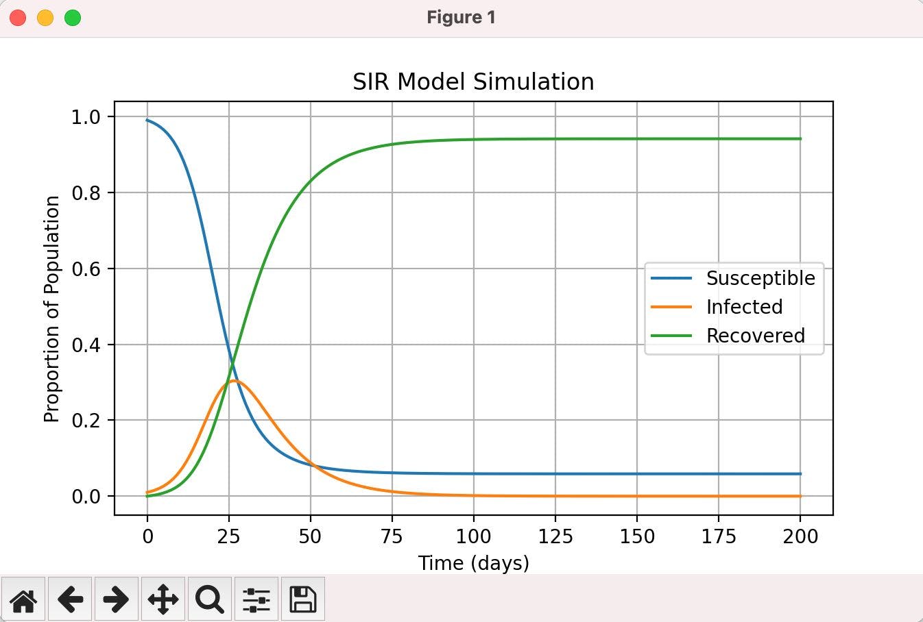
- Understand Disease Spread: Observe the epidemic curve and visualize how a disease spreads through a community. Running Python SIR Model above, you can see the outcome/result in the graph below:
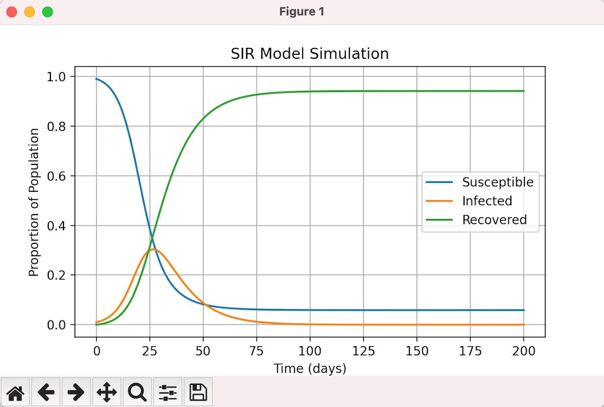
Result of our simulation showing reduced susceptibility, and infection rate, with high recovery rates.
- Explore Parameter Sensitivity:Try testing various beta and gamma values to observe how they affect the length and peak of the outbreak.
- Evaluate Interventions:By changing the parameters, you can simulate the consequences of interventions likesocial isolation or immunization.
3. The SEIR Model
What It Does / SEIR Python Code Simulation Example
By adding a “Exposed” compartment, the SEIR model expands upon the SIR model. It takes into account the period of incubation during which people have been exposed but are not yet contagious. How to emulate it in Python is shown here.
import numpy as np
from scipy.integrate import odeint
import matplotlib.pyplot as plt

# SEIR model equations
def SEIR_model(y, t, beta, sigma, gamma):
    S, E, I, R = y
    dSdt = -beta * S * I
    dEdt = beta * S * I - sigma * E
    dIdt = sigma * E - gamma * I
    dRdt = gamma * I
    return [dSdt, dEdt, dIdt, dRdt]

# Initial conditions
S0 = 0.99
E0 = 0.01
I0 = 0.00
R0 = 0.00
y0 = [S0, E0, I0, R0]

# Parameters
beta = 0.3
sigma = 0.1
gamma = 0.05

# Time vector
t = np.linspace(0, 200, 200)

# Solve the SEIR model equations
solution = odeint(SEIR_model, y0, t, args=(beta, sigma, gamma))

# Extract results
S, E, I, R = solution.T

# Plot the results
plt.figure(figsize=(10, 6))
plt.plot(t, S, label='Susceptible')
plt.plot(t, E, label='Exposed')
plt.plot(t, I, label='Infected')
plt.plot(t, R, label='Recovered')
plt.xlabel('Time (days)')
plt.ylabel('Proportion of Population')
plt.title('SEIR Model Simulation')
plt.legend()
plt.grid(True)
plt.show()
The only difference in this case is the introduction of latent period rate (?) to explore different scenarios and understand the dynamics of infectious diseases with an “exposed” period. It demonstrates how it accounts for an incubation period before individuals become infectious.
What You Can Learn
When you use Python to run the SEIR model, you can:
- Model Latent PeriodsRecognize the differences between the behaviors of immediately infectious illnesses and diseases with incubation periods.
- Evaluate Early InterventionsAnalyze the effects of isolation and early detection strategies.
- Study Complex OutbreaksFor illnesses like COVID-19 where exposed people are a major factor in transmission, use SEIR.
4. Conclusion
Python’s simplicity and robust libraries, like SciPy, make it the perfect language for modeling diseases. And by performing these simulations with it, you’re learning more about the dynamics of infectious diseases. This can equip you with verdicts and prowess that can help make decisions that are well-informed and improve your own ability to evaluate epidemics in the real world.
There is much more to come after the SIR and SEIR models. There are other complex models such as SEIRS (Susceptible-Exposed-Infectious-Removed-Susceptible) Model, Spatial Models, Network Models, etc. Investigating intricate models, as well as real world data, such as geospatial data, epidemiological data, behavioural data, etc, and carefully examining the effects of interventions, such as vaccination strategies, treatment availability, social distancing measures, you will develop your modeling abilities even further.
Your knowledge of these modeling tools can significantly impact protecting public health in a future where understanding infectious disease transmission is vital.
This is already too long, but I hope I have been able to show you how to simulate SIR and SEIR Models in mathematical model, using Python.
This article was originally published by Olaoluwa Afolabi on Hackernoon.


